Modeling Correlated RV Variability With A Gaussian Process

This tutorial focuses on the harv.GP extension for radial-velocity data. A Gaussian process (GP) lets us model correlated stellar variability or instrumental systematics that are not well described by independent per-epoch noise terms.

We assume you have already worked through the getting started tutorial and the MCMC continuation tutorial. Here we first use the rejection sampler to find promising regions of parameter space for a GP-extended model, then warm-start harv.NumpyroSampler to refine the posterior with MCMC.

import astropy.table as at
import jax
import matplotlib.pyplot as plt
import numpyro.distributions as dist
import quaxed.numpy as jnp
from unxt import Q

import harv
import harv.models as hm

jax.config.update("jax_enable_x64", True)

%matplotlib inline

GP model for stellar variability

Jitter is the simplest noise extension, but it assumes the excess noise is uncorrelated in time. Many real (and astrophysical) noise sources are not. Red giants, in particular, show RV variability on timescales of hours to weeks driven by convective granulation and surface oscillations. This produces correlated residuals, and treating that with a single jitter parameter inflates the error budget on short timescales and on long timescales in different ways.

The GP extension adds a GP covariance term \(K(t, t')\) to the RV likelihood. In harv, you specify the GP through a kernel_builder(hp) callable that returns a tinygp kernel for one set of hyper-parameters.

For this section we use a low surface gravity (LOGG) APOGEE red giant branch (RGB) source.

tbl = at.Table.read("../data/apogeedr17-2M02372118-3437451.csv")
rgb_data = harv.RVData(
    time=Q(tbl["JD"].astype("f8"), "day"),
    rv=Q(tbl["VHELIO"].astype("f8"), "km/s"),
    rv_err=Q(tbl["VRELERR"].astype("f8"), "km/s"),
)
_ = rgb_data.plot(relative_to_t_ref=True)

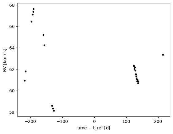
This source has a logg = 0.66 (as measured by APOGEE), which probably corresponds to having variability on timescales of ~20–30 days or so. The radial velocity trends we see in the data are probably dominated by this stellar variability, but we can use harv with the Keplerian model + a GP to see if we can constrain any additional Keplerian signals in the data.

Building the GP extension

For this example we use the damped simple harmonic oscillator (SHO) kernel implemented in tinygp.kernels.quasisep.SHO. This is a good match to stochastic red-giant variability, and tinygp provides an efficient quasiseparable implementation of this kernel.

The GP extension needs:

• a kernel_builder() callable that takes a dict of (unit-stripped) hyper-parameter values and returns a tinygp kernel;

• a list of ParamInfo declarations for the hyper-parameters (these become nonlinear parameters that the rejection sampler draws from their priors); and

• a time_unit string telling the extension what unit to strip times to before evaluating the kernel.

We will parameterize the kernel with:

• gp_omega — characteristic angular frequency in 1/day;

• gp_Q — quality factor (dimensionless); and

• gp_sigma — GP amplitude in km/s.

Note that tinygp is an optional dependency of harv; you can install it directly, or via pip install "harv[extra]", or uv add "harv[extra]".

import tinygp

def rgb_kernel(params):
    return tinygp.kernels.quasisep.SHO(
        omega=params["gp_omega"], quality=params["gp_Q"], sigma=params["gp_sigma"]
    )


gp_ext = harv.GP(
    kernel_builder=rgb_kernel,
    hyperparams=(
        harv.ParamInfo("gp_omega", "1/day"),
        harv.ParamInfo("gp_Q", ""),
        harv.ParamInfo("gp_sigma", "km/s"),
    ),
    time_unit="day",
)

The GP hyperparameter priors attach to the prior the same way as jitter, by passing them as keyword arguments to default_rv. Here we use log-normal priors on gp_omega and gp_Q, and a half-normal prior on gp_sigma. Because the GP extension adds three nonlinear hyperparameters, the rejection sampler is mainly serving as a fast way to find high-likelihood starting points for MCMC.

model_gp = harv.RVModel(extensions=(gp_ext,))

prior_gp = hm.StandardRV().default_prior(
    period_min=Q(20.0, "day"),
    period_max=Q(3000.0, "day"),
    sigma_K0=Q(30.0, "km/s"),
    sigma_v0=Q(50.0, "km/s"),
    gp_omega=harv.QD(dist.LogNormal(0.0, 2.0), "1/day"),
    gp_Q=harv.QD(dist.LogNormal(2.0, 1.5), ""),
    gp_sigma=harv.QD(dist.HalfNormal(1.0), "km/s"),
)

sampler_gp = harv.RejectionSampler(
    prior_gp,
    model_gp,
)
samples_gp = sampler_gp.run(
    rgb_data,
    n_prior_samples=1_000_000,
    max_posterior_samples=512,
    seed=42,
    ignore_non_finite=True,  # sometimes the GP can produce nan values
)
len(samples_gp)

42

Once we have a set of accepted GP-extended samples, we can warm-start NUTS from them. This is often the most practical workflow for GP models: use rejection sampling to locate the interesting part of parameter space, then let MCMC map the local posterior structure in more detail.

For this tutorial we keep the MCMC run modest and use two sequential chains to reduce notebook resource usage.

mcmc_gp = harv.NumpyroSampler(prior_gp, model_gp)
samples_gp_mcmc = mcmc_gp.run(
    rgb_data,
    init_samples=samples_gp,
    seed=43,
    num_chains=2,
    num_warmup=200,
    num_samples=100,
    chain_method="sequential",
)
samples_gp_mcmc.n_samples

200

samples_gp_mcmc.keys()

['period',
 'eccentricity',
 'phase_peri',
 'arg_peri',
 'gp_omega',
 'gp_Q',
 'gp_sigma',
 'rv_semiamp',
 'v_sys',
 'log_period',
 't_peri',
 'binary_mass_function']

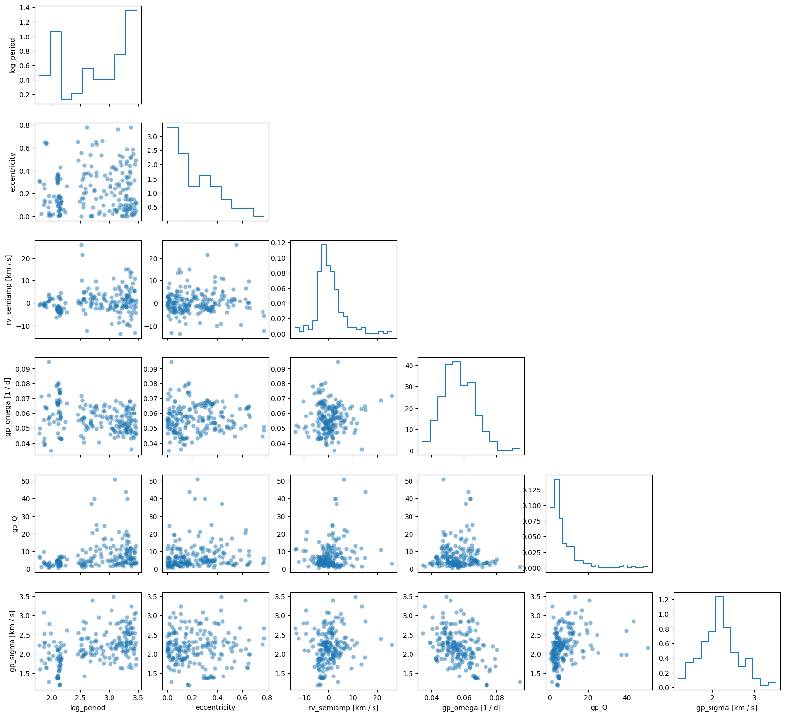
_ = samples_gp_mcmc.plot_corner(
    ["log_period", "eccentricity", "rv_semiamp", "gp_omega", "gp_Q", "gp_sigma"]
)

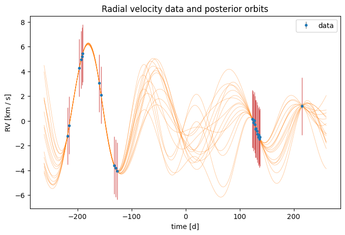
We can now visualize the MCMC-refined posterior in the time domain. When we pass the GP extension to harv.plot.plot_rv, the plot shows the GP conditional-mean contribution on top of the Keplerian orbit overlays:

fig, ax = plt.subplots(figsize=(8, 5))
ax = harv.plot.plot_rv(
    samples_gp_mcmc,
    data=rgb_data,
    model=model_gp,
    n_samples=16,
    relative_to_t_ref=True,
    relative_to_median_v_sys=True,
    ax=ax,
)

We can also use plot_rv to visualize the Keplerian and non-Keplerian (here, GP) contributions to the RVs separately:

fig, ax = plt.subplots(figsize=(8, 5))
ax = harv.plot.plot_rv(
    samples_gp_mcmc,
    data=rgb_data,
    model=model_gp,
    n_samples=16,
    relative_to_t_ref=True,
    relative_to_median_v_sys=True,
    show_signal_components=True,
    ax=ax,
)

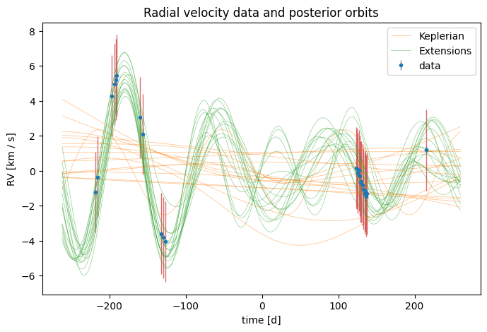
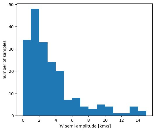
Here we can see that the GP can plausibly explain all of the RV variability we see in the data, and the Keplerian contribution is consistent with zero amplitude:

fig, ax = plt.subplots(figsize=(6, 5))
ax.hist(jnp.abs(samples_gp_mcmc["rv_semiamp"]).value, bins=jnp.linspace(0, 15.0, 16))
ax.set(xlabel="RV semi-amplitude [km/s]", ylabel="number of samples")

[Text(0.5, 0, 'RV semi-amplitude [km/s]'), Text(0, 0.5, 'number of samples')]