Modeling SB2 radial velocity data

In this tutorial, we model radial velocities for a double-lined spectroscopic binary (SB2), where we have measured RVs for both components of the binary. Constructing a model for an SB2 requires one additional step compared to the SB1 workflow: we must create a harv.JointModel object to pass to the sampler that tells the sampler to share parameters across components of the model (i.e., period is the same for both stars in an SB2). The nonlinear orbital parameters are shared between the two components, while each component keeps its own RV semi-amplitude and jitter term.

The key differences from the SB1 workflow are:

1. We store the two RV time series in a harv.data.SystemData container instead of a single harv.data.RVData instance,

2. We construct a harv.JointModel using the harv.JointModel.for_sb2() constructor to join the likelihoods for the two components (primary and secondary) of the system.

3. We include a jitter parameter for each component with the harv.Jitter extension.

4. We use the rejection sampler output to start an MCMC continuation with harv.NumpyroSampler.

This tutorial assumes that you have read through the getting started tutorial and are familiar with the basic rejection-sampling workflow for single-lined RV data.

import astropy.table as at
import jax
import numpyro.distributions as dist
import quaxed.numpy as jnp
from cycler import cycler
from unxt import Q

import harv

jax.config.update("jax_enable_x64", True)

%matplotlib inline

Loading the SB2 radial velocity data

For this example, we will use APOGEE RV measurements for a known SB2 system. This data comes from Kounkel et al. 2021, which provides separate RV measurements for the primary and secondary components. We build a harv.RVData object for each component and place them in a harv.data.SystemData container:

tbl = at.Table.read("../data/apogee-KounkelSB2-2M13481613-0510559.csv")

# Make sure the data is f64
fdtype = jnp.float64

primary_data = harv.RVData(
    time=Q(tbl["HJD"].astype(fdtype), "day"),
    rv=Q(tbl["RVel1"].astype(fdtype), "km/s"),
    rv_err=Q(jnp.abs(tbl["e_RVel1"].astype(fdtype)), "km/s"),
)

secondary_tbl = tbl[~tbl["RVel2"].mask].filled()
secondary_data = harv.RVData(
    time=Q(secondary_tbl["HJD"].astype(fdtype), "day"),
    rv=Q(secondary_tbl["RVel2"].astype(fdtype), "km/s"),
    rv_err=Q(jnp.abs(secondary_tbl["e_RVel2"].astype(fdtype)), "km/s"),
)

Now we combine the two datasets into a SystemData object, which is the expected input for modeling SB2s. There is nothing special about the names “primary” and “secondary” here - you can use whatever names you like:

data = harv.data.SystemData(
    primary=primary_data,
    secondary=secondary_data,
)

list(data.keys())

['primary', 'secondary']

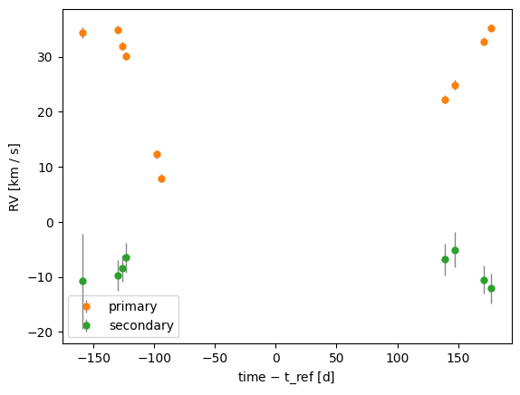
Let’s start by plotting the data:

_ = data.plot(
    relative_to_t_ref=True, color_cycler=cycler(color=["C1", "C2"]), markersize=5
)

Building a joint SB2 model in harv

For an SB2, both components share the same nonlinear orbital parameters and the systemic velocity, but each component has its own RV semi-amplitude and its own jitter term. We can use the harv.default_sb2_prior() helper to construct the shared nonlinear priors for a typical SB2 model, and then use the harv.JointModel.for_sb2 constructor to build a joint model for simultaneously modeling the two components:

prior = harv.models.default_sb2_prior(
    period_min=Q(1.0, "day"),
    period_max=Q(3000.0, "day"),
    sigma_K0=Q(120.0, "km/s"),
    sigma_v0=Q(100.0, "km/s"),
    **{
        "primary.jitter": harv.QD(dist.HalfNormal(1.0), "km/s"),
        "secondary.jitter": harv.QD(dist.HalfNormal(1.0), "km/s"),
    },
)

exts = {"primary": (harv.Jitter("km/s"),), "secondary": (harv.Jitter("km/s"),)}
joint_model = harv.JointModel.for_sb2(prior, extensions=exts)

Let’s inspect the structure of the prior. The four shared orbital parameters live in nonlinear_priors. The linear_prior dict contains the per-component semi-amplitudes (primary.rv_semiamp, secondary.rv_semiamp) and the shared systemic velocity (v_sys).

(
    prior.nonlinear_priors.keys(),
    prior.linear_priors.keys(),
    prior.extension_priors.keys(),
)

(dict_keys(['period', 'eccentricity', 'phase_peri', 'arg_peri']),
 dict_keys(['primary.rv_semiamp', 'secondary.rv_semiamp', 'v_sys']),
 dict_keys(['primary.jitter', 'secondary.jitter']))

Rejection sampling

With the SB2 joint model in hand, we can run the rejection sampler exactly as in the SB1 case. The linear parameters are still marginalized analytically inside each RV component model.

rejection_sampler = harv.RejectionSampler(prior, joint_model)

rejection_samples = rejection_sampler.run(
    data,
    n_prior_samples=10_000_000,
    max_posterior_samples=1024,
    seed=42,
)

rejection_samples

Samples(n_samples=6, data_type='JointModel', parameters=11)

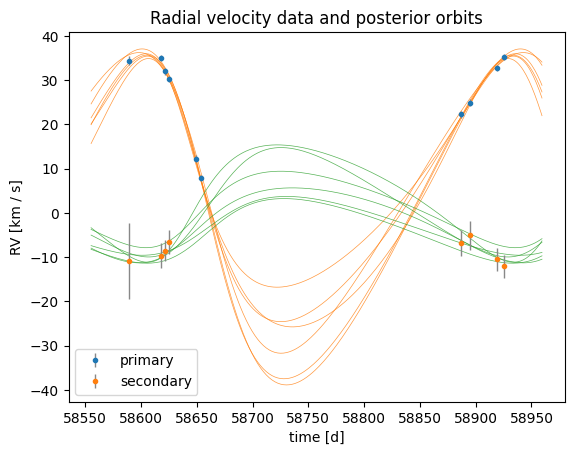
The returned harv.Samples object contains the four shared nonlinear orbital parameters, the two component-specific jitter parameters, and namespaced linear parameters for the two RV components (primary.rv_semiamp, secondary.rv_semiamp) plus the shared v_sys. harv.plot.plot_rv() understands the SystemData container and draws posterior orbits over the data for each component automatically, so a single call gives us a quick visual check that the rejection-sampler modes are sensible:

_ = harv.plot.plot_rv(rejection_samples, data)

Wrapping the angles and sign convention for semi-amplitudes

In order to enable marginalization over the linear parameters, the rejection sampler uses Gaussian priors on each component’s rv_semiamp that are symmetric about zero. This means that the semi-amplitudes can be positive or negative. The posterior for an SB2 therefore contains two equivalent sign conventions:

• \((K_1 > 0,\; K_2 < 0,\; \omega)\) — primary moving toward us at periastron, secondary moving away,

• \((K_1 < 0,\; K_2 > 0,\; \omega + \pi)\) — exactly the same physical orbit, opposite labelling.

These correspond to the same orbit; the two K’s are anti-correlated and “lock” their signs together via the shared argument of periastron \(\omega\). Calling harv.Samples.wrap_angles() collapses both forms onto the canonical convention \(K_1 \ge 0\) by flipping the signs of every rv_semiamp-suffixed key (and shifting the shared arg_peri by \(\pi\)) for the negative-trigger samples.

Note

In some cases, when \(K_2\) is small or unconstrained, you can end up with unphysical posterior samples in which both \(K_1\) and \(K_2\) have the same sign. These orbits are not possible, but are a consequence of the Gaussian marginalization over a symmetric prior on \(K\). In those cases, you can either run with many more prior samples and reject the cases where sign(K_1) == sign(K_2) or make \(K_2\) an explicitly sampled parameter so you can control the sign of the parameter.

wrapped_samples = rejection_samples.wrap_angles()

Continuing with MCMC using NumpyroSampler

Once the rejection sampler has identified the relevant posterior modes, if the posterior is uniform in period, we can use those posterior samples to start a more standard MCMC sampling. This is especially useful for refining local structure within the accepted modes. NumpyroSampler requires the rejection-sampler output as init_samples.

However, we rebuild the prior with two adjustments for the MCMC continuation. First, now that we’ve used wrap_angles() to put the rejection samples in the canonical \(K_1 \ge 0\) mode, we switch to sign-restricted priors on the semi-amplitudes so the NUTS chains don’t waste warmup drifting back into the equivalent flipped-sign mode:

• primary.rv_semiamp ~ HalfNormal(100 km/s) — positive support only,

• secondary.rv_semiamp ~ TruncatedNormal(scale=100 km/s, high=0) — negative support only.

Second, with non-Gaussian priors on the semi-amplitudes, those parameters are no longer analytically marginalizable and will instead be sampled explicitly by the MCMC kernel; the shared v_sys (which kept its Gaussian prior) is still marginalized, as you’ll see in a warning printed by the sampler.

mcmc_prior = harv.models.default_sb2_prior(
    period_min=Q(1.0, "day"),
    period_max=Q(3000.0, "day"),
    sigma_v0=Q(100.0, "km/s"),
    **{
        "primary.rv_semiamp": harv.QD(dist.HalfNormal(100.0), "km/s"),
        "secondary.rv_semiamp": harv.QD(
            dist.TruncatedNormal(scale=100.0, high=0.0), "km/s"
        ),
        "primary.jitter": harv.QD(dist.HalfNormal(5.0), "km/s"),
        "secondary.jitter": harv.QD(dist.HalfNormal(5.0), "km/s"),
    },
)

mcmc_joint_model = harv.JointModel.for_sb2(mcmc_prior, extensions=exts)

numpyro_sampler = harv.NumpyroSampler(mcmc_prior, mcmc_joint_model)

mcmc_samples = numpyro_sampler.run(
    data,
    init_samples=wrapped_samples,
    seed=42,
    num_chains=2,
    num_warmup=500,
    num_samples=500,
    chain_method="sequential",
)

mcmc_samples

/home/runner/work/harv/harv/src/harv/samplers/numpyro.py:366: UserWarning: Non-Gaussian linear prior(s) ['primary.rv_semiamp', 'secondary.rv_semiamp'] cannot be analytically marginalized and will be sampled explicitly. Marginalized parameters: ('v_sys',)
  prepared = _prepare_sampler_model(

Samples(n_samples=1000, data_type='JointModel', parameters=11)

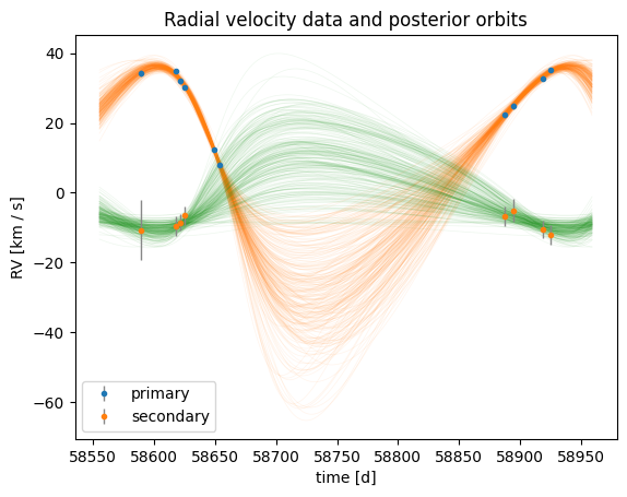
As before, we visualize the posterior orbits over the data. Compared to the rejection-sampler view, the curves should be visibly tighter — NUTS has explored the local geometry of each accepted mode in detail rather than just sampling individual draws from it.

_ = harv.plot.plot_rv(mcmc_samples, data, n_samples=256)

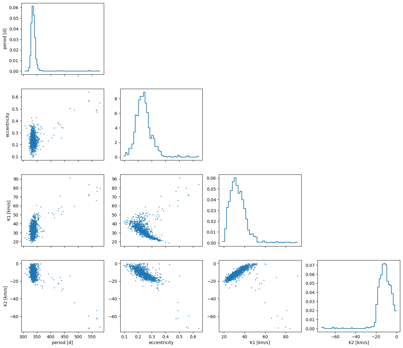
We now make a corner plot of the physical parameters: the two semi-amplitudes, period, and eccentricity. This reveals the structure of the joint SB2 posterior pdf. Two features are characteristic of well-fit SB2 systems:

1. A tight, narrow K_1/K_2 “ridge”: The two semi-amplitudes are correlated and constrain well the binary mass ratio \(q = M_2 / M_1 = K_1 / |K_2|\), so the joint posterior collapses onto a thin diagonal band.

2. A well-defined period mode: Unlike the often multimodal posterior of a single-lined RV fit, observing both stars simultaneously usually pins the period much more tightly.

corner_keys = ["period", "eccentricity", "primary.rv_semiamp", "secondary.rv_semiamp"]

pm = mcmc_samples.plot_corner(
    corner_keys,
    figure_kwargs={"figsize": (16, 14)},
    visuals={"scatter": {"alpha": 0.8, "s": 6}},
    labels={"primary.rv_semiamp": "K1 [km/s]", "secondary.rv_semiamp": "K2 [km/s]"},
)