Customizing the prior distributions and changing parametrization

NOTE: This tutorial assumes that you have read through the getting started tutorial and are familiar with the basic rejection-sampling workflow.

In this tutorial, we show how to customize the prior distributions and change the parametrization of the model.

import astropy.table as at
import jax
import matplotlib.pyplot as plt
import numpyro.distributions as dist
import quaxed.numpy as jnp
from unxt import Q, ustrip

import harv
import harv.models as hm

jax.config.update("jax_enable_x64", True)

%matplotlib inline

For this tutorial we will use the same data as in the getting started tutorial, but we will show the impact of changing the priors and parametrization on the returned posterior samples.

tbl = at.Table.read("../data/apogeedr17-2M17155561-4203387.csv")

fdtype = jnp.float64
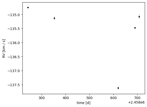
data = harv.RVData(
    time=Q(tbl["JD"].astype(fdtype), "day"),
    rv=Q(tbl["VHELIO"].astype(fdtype), "km/s"),
    rv_err=Q(tbl["VRELERR"].astype(fdtype), "km/s"),
)
_ = data.plot()

Customizing the prior

The default RV prior in harv assumes a log-uniform period distribution and the eccentricity prior from Kipping (2013):

default_prior = hm.StandardRV().default_prior(
    period_min=Q(0.5, "day"),
    period_max=Q(3000.0, "day"),
    sigma_K0=Q(30.0, "km/s"),
    sigma_v0=Q(50.0, "km/s"),
)

Let’s start by using this prior to generate posterior samples for our data, as a baseline:

run_kwargs = {
    "n_prior_samples": 10_000_000,
    "max_posterior_samples": 512,
    "seed": 42,
}
default_samples = harv.RejectionSampler(default_prior, harv.RVModel()).run(
    data, **run_kwargs
)
len(default_samples)

67

Any of the default priors can be overridden by passing a custom prior distribution to the HarvPrior constructor. For example, we could instead use a Gaussian period distribution and a uniform eccentricity distribution:

norm_unif_prior = hm.StandardRV().default_prior(
    period=harv.QD(dist.TruncatedNormal(500.0, 50.0, low=0.0), "day"),
    eccentricity=dist.Uniform(0.0, 1.0),
    sigma_K0=Q(30.0, "km/s"),
    sigma_v0=Q(50.0, "km/s"),
)

norm_unif_samples = harv.RejectionSampler(norm_unif_prior, harv.RVModel()).run(
    data, **run_kwargs
)
len(norm_unif_samples)

512

fig, ax = plt.subplots(figsize=(8, 5))
ax = harv.plot.plot_rv(
    norm_unif_samples,
    data=data,
    n_samples=128,
    relative_to_t_ref=True,
    relative_to_median_v_sys=True,
    ax=ax,
)

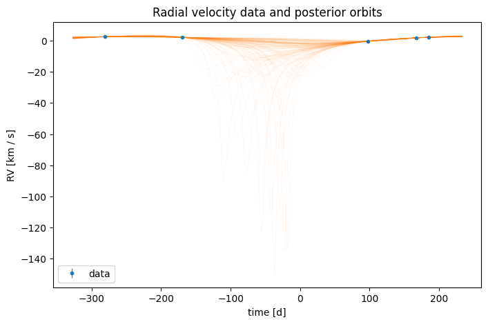
You can also use these overrides to set a fixed value for a parameter using the numpyro Delta distribution. For example, if we wanted to fix the eccentricity to zero, we could set eccentricity=dist.Delta(0.0) in the prior:

fixed_ecc0_prior = hm.StandardRV().default_prior(
    period_min=Q(0.5, "day"),
    period_max=Q(3000.0, "day"),
    eccentricity=dist.Delta(0.0),
    sigma_K0=Q(30.0, "km/s"),
    sigma_v0=Q(50.0, "km/s"),
)

fixed_ecc0_samples = harv.RejectionSampler(fixed_ecc0_prior, harv.RVModel()).run(
    data, **run_kwargs
)
len(fixed_ecc0_samples)

230

fig, ax = plt.subplots(figsize=(8, 5))
ax = harv.plot.plot_rv(
    fixed_ecc0_samples,
    data=data,
    n_samples=512,
    relative_to_t_ref=True,
    relative_to_median_v_sys=True,
    ax=ax,
)

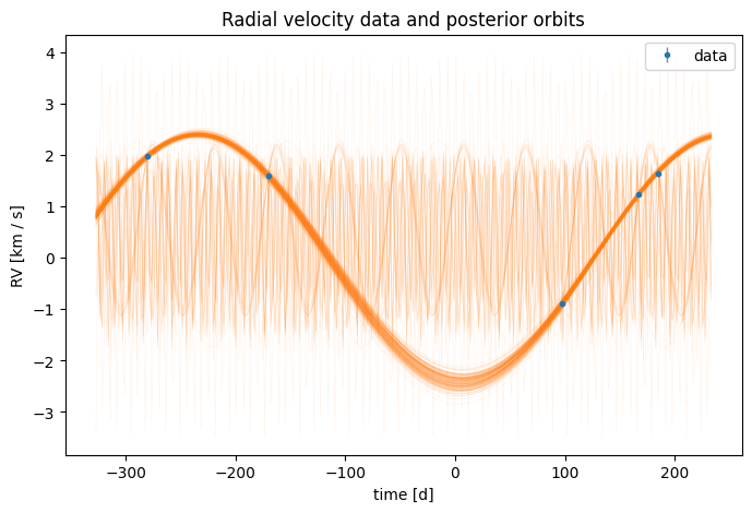
If you prefer to override all of the default priors, you can also construct a HarvPrior directly from a dictionary of parameter names and prior distributions: The default_prior helper methods provide a convenient way to construct the standard RV priors without having to specify each one individually, but you can also construct the same prior by hand:

fully_custom_prior = harv.HarvPrior(
    nonlinear_priors={
        "period": harv.QD(dist.TruncatedNormal(500.0, 10.0, low=0.0), "day"),
        "eccentricity": dist.Uniform(0.0, 0.5),
        "arg_peri": harv.QD(dist.Uniform(0.0, 360.0), "degree"),
        "phase_peri": dist.Uniform(0.0, 1.0),
    },
    linear_priors={
        "rv_semiamp": harv.QD(dist.Normal(0.0, 10.0), "km/s"),
        "v_sys": harv.QD(dist.Normal(-135.0, 10.0), "km/s"),
    },
)

fully_custom_samples = harv.RejectionSampler(fully_custom_prior, harv.RVModel()).run(
    data, **run_kwargs
)
len(fully_custom_samples)

512

fig, ax = plt.subplots(figsize=(8, 5))
ax = harv.plot.plot_rv(
    fully_custom_samples,
    data=data,
    n_samples=512,
    relative_to_t_ref=True,
    relative_to_median_v_sys=True,
    ax=ax,
)

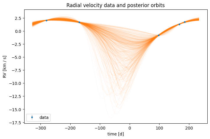
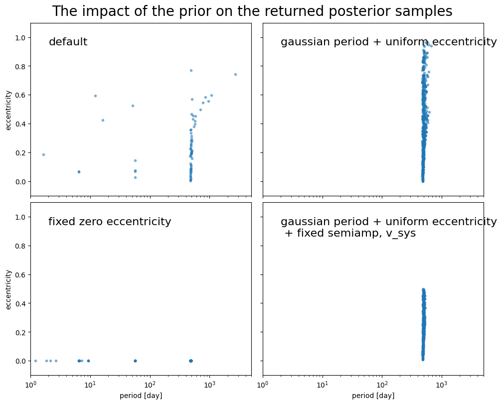
The impact of the prior on the returned posterior samples

As you can see from the orbit plots above, the choice of prior has a significant impact on the returned posterior samples for weakly-constraining data (e.g., low signal-to-noise, few epochs, or sparse sampling).

all_samples = {
    "default": default_samples,
    "gaussian period + uniform eccentricity": norm_unif_samples,
    "fixed zero eccentricity": fixed_ecc0_samples,
    (
        "gaussian period + uniform eccentricity\n + fixed semiamp, v_sys"
    ): fully_custom_samples,
}

fig, axes = plt.subplots(
    2, 2, figsize=(10, 8), sharex=True, sharey=True, layout="constrained"
)

for ax, (name, samples) in zip(axes.flat, all_samples.items(), strict=False):
    ax.plot(
        ustrip("day", samples["period"]),
        samples["eccentricity"],
        marker=".",
        linestyle="none",
        alpha=0.5,
    )
    ax.text(2, 1.0, name, ha="left", va="top", fontsize=16)

for ax in axes[:, 0]:
    ax.set_ylabel("eccentricity")
for ax in axes[-1, :]:
    ax.set_xlabel("period [day]")

ax.set(xlim=(1e0, 5e3), xscale="log", ylim=(-0.1, 1.1))
fig.suptitle("The impact of the prior on the returned posterior samples", fontsize=20)

Text(0.5, 0.98, 'The impact of the prior on the returned posterior samples')

---

Changing which parameters are marginalized

By default, the rejection sampler analytically marginalizes over both linear RV parameters, rv_semiamp and v_sys. You can override this behavior by passing marginalized_names when constructing the sampler.

In the example below, we set marginalized_names=("rv_semiamp",), so the RV semiamplitude remains analytically marginalized while the systemic velocity is sampled explicitly during the rejection step. Because v_sys is now drawn directly from its prior, it helps to choose a prior centered near the observed mean RV for this source.

explicit_vsys_prior = hm.StandardRV().default_prior(
    period_min=Q(0.5, "day"),
    period_max=Q(3000.0, "day"),
    sigma_K0=Q(30.0, "km/s"),
    v_sys=harv.QD(dist.Cauchy(-137.0, 10.0), "km/s"),
)

sampler_only_k = harv.RejectionSampler(
    explicit_vsys_prior,
    harv.RVModel(),
    marginalized_names=("rv_semiamp",),
)

explicit_vsys_samples = sampler_only_k.run(
    data,
    n_prior_samples=10_000_000,
    max_posterior_samples=512,
    seed=45,
)
len(explicit_vsys_samples)

3

However, note that this can lead to a significant increase in the number of prior samples needed to get a given number of posterior samples (i.e., this can hurt the acceptance rate), because the parameter dimensionality increases.