Getting started: Modeling radial velocity (RV) data

harv is a JAX-native Python package for inferring Keplerian orbital parameters of binary star or star–exoplanet systems. harv provides a rejection sampler that implements analytic marginalization over linear parameters to improve the efficiency of the sampling, along with extensions to support continued sampling with MCMC. harv is an evolution of the rejection sampler implemented in The Joker, so see Key concepts in harv and the original paper for more details about the method.

This tutorial covers basic functionality around modeling RV data, including:

• Creating a RVData object,

• Setting up a HarvPrior with the default prior distributions and parameterization,

• Running the RejectionSampler to get posterior samples, and

• Visualizing the results.

Other tutorials demonstrate more advanced functionality:

• Customizing the prior distributions

• Extending the model with extra noise terms, trends, or instrumental offsets

• Continuing the posterior sampling with numpyro

• Modeling SB2 systems

Let’s start with the imports we’ll need:

import astropy.table as at
import jax
import matplotlib.pyplot as plt
import quaxed.numpy as jnp
from unxt import Q

import harv
import harv.models as hm

jax.config.update("jax_enable_x64", True)

%matplotlib inline

Loading radial velocity data

The main data container for RV data in harv is harv.RVData, which stores barycentric observation times, measured radial velocities, and uncertainties. These are all specified as unxt.Quantity objects with explicit physical units, which is like the more familiar astropy.units.Quantity but with support for JAX transformations. See the unxt documentation for more details. In unxt, it is standard to use the short-hand alias Q for unxt.Quantity, which we do for brevity below. Since jax.numpy doesn’t know how to handle unxt.Quantity objects, we use quaxed.numpy (imported as jnp) for any mathematical operations - see the unxt documentation or the sharp bits page for more information about working with unxt and jax.

For this tutorial, we will use RV data from the APOGEE survey data release 17 (DR17) for a source (APOGEE_ID=2M17155561-4203387) with only 5 observations. We deliberately choose a source with few observations to demonstrate the power of the rejection sampling method.

tbl = at.Table.read("../data/apogeedr17-2M17155561-4203387.csv")

fdtype = jnp.float64
data = harv.RVData(
    time=Q(tbl["JD"].astype(fdtype), "day"),
    rv=Q(tbl["VHELIO"].astype(fdtype), "km/s"),
    rv_err=Q(tbl["VRELERR"].astype(fdtype), "km/s"),
)
data

RVData(
  time=Quantity(f64[5], unit='d'),
  t_ref=Quantity(weak_f64[], unit='d'),
  rv=Quantity(f64[5], unit='km / s'),
  rv_err=Quantity(f64[5], unit='km / s')
)

Let’s start by plotting the data:

_ = data.plot(relative_to_t_ref=True)

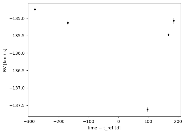
The data are clearly variable, but with only a few observations, many orbital periods and orbital solutions should be consistent with the data. The rejection sampler in harv will enable us to map out this multi-modal posterior.

Specifying the prior distributions

With data in hand, our next task is to set up the prior probability distribution for rejection sampling. The default prior for radial velocity data can be initialized using the default_prior() class method of harv.models.StandardRV, which sets up a log-uniform period prior, the Kipping (2013) eccentricity prior, along with uniform priors on the phase and argument of periastron. The linear parameters (RV semi-amplitude and systemic velocity) are marginalized out analytically, with a Gaussian prior whose width (in semi-amplitude) scales with period and eccentricity to keep it approximately constant in companion mass.

Here, period_min and period_max set the minimum and maximum periods for the default log-uniform period prior, sigma_K0 sets the scale factor for the Gaussian prior on the RV semi-amplitude at the reference period P0 (by default 1 year, but this can be configured by changing P0), and sigma_v0 sets the (fixed) width of the Gaussian prior on the systemic velocity. The default values for these parameters are set to be broadly appropriate for stellar companions, but they can be customized as needed (for example, to be more appropriate for exoplanet companions) - see the next tutorial for more details.

prior = hm.StandardRV().default_prior(
    period_min=Q(0.5, "day"),
    period_max=Q(3000, "day"),
    sigma_K0=Q(30.0, "km/s"),
    sigma_v0=Q(50.0, "km/s"),
)

Let’s see the breakdown of which parameters are included in the nonlinear and linear priors using the default prior setup:

print(prior.nonlinear_priors.keys())
print(prior.linear_priors.keys())

dict_keys(['period', 'eccentricity', 'phase_peri', 'arg_peri'])
dict_keys(['rv_semiamp', 'v_sys'])

The prior has four nonlinear parameters (period, eccentricity, orbital phase, argument of periastron). The linear parameters are rv_semiamp or \(K\) and v_sys or \(v_0\).

Running the rejection sampler

With data and prior now specified, we can create a harv.RejectionSampler to manage running the rejection sampling:

sampler = harv.RejectionSampler(prior, harv.RVModel())

And then we can call .run() to run the sampler. The default specification for the sampler requires the number of prior samples to draw (n_prior_samples) and the maximum number of posterior samples to return (max_posterior_samples). You can also set a random number seed (seed) for reproducibility.

samples = sampler.run(
    data,
    n_prior_samples=10_000_000,
    max_posterior_samples=1024,
    seed=42,
)
samples

Samples(n_samples=67, data_type='RVModel', parameters=9)

The returned Samples object behaves like a Python dictionary: you can access parameter values by name as keys and the sample values are returned as unxt.Quantity objects with units, for example:

samples["period"]

[5.66183371e+01, 4.89877840e+02, 4.83538602e+02, 4.95603713e+02, 4.86166647e+02, 1.63386137e+00, 4.93778171e+02, 5.44913047e+02, 9.62432019e+02, 4.92942563e+02, 4.91898195e+02, 4.95608438e+02, 5.66382186e+01, 5.10612420e+01, 4.79703246e+02, 4.77525366e+02, 4.87740865e+02, 4.71086363e+02, 4.76692315e+02, 4.84268586e+02, 4.85083033e+02, 5.23502988e+02, 4.96310368e+02, 5.75660797e+02, 4.84331682e+02, 6.47810168e+00, 1.06392140e+03, 5.72686189e+02, 4.78469207e+02, 6.47790802e+00, 1.20036336e+01, 4.84724685e+02, 5.66316708e+01, 5.64285671e+02, 5.66945473e+01, 4.81510674e+02, 5.05647665e+02, 4.95267879e+02, 4.79768147e+02, 4.79090610e+02, 4.81803320e+02, 4.82263106e+02, 5.21758712e+02, 4.81566229e+02, 4.74199561e+02, 4.84478277e+02, 4.75725400e+02, 4.96526167e+02, 8.49163532e+02, 4.91918423e+02, 4.81267835e+02, 2.67579751e+03, 4.90740474e+02, 4.86341704e+02, 5.07537771e+02, 1.61293599e+01, 5.04720620e+02, 4.87150059e+02, 4.83078013e+02, 7.77975240e+02, 4.85501066e+02, 4.88827127e+02, 4.77303549e+02, 4.78440045e+02, 5.07730587e+02, 4.90106178e+02, 7.04471376e+02] * Unit("d")

Working with and visualizing the returned posterior samples

I find it useful to first look at the returned posterior samples to get a sense of the structure of the posterior and the types of orbits that are consistent with the data. As a first visualization, we can use the Samples.plot_corner() method to make a corner plot of the posterior samples:

axes = samples.plot_corner(
    ["period", "eccentricity", "rv_semiamp", "v_sys"],
    visuals={"scatter": {"alpha": 0.75, "s": 2}},
)
for ax in axes.viz["plot"].isel(col_index=0).values.flat:
    if ax is not None:
        ax.set_xscale("log")

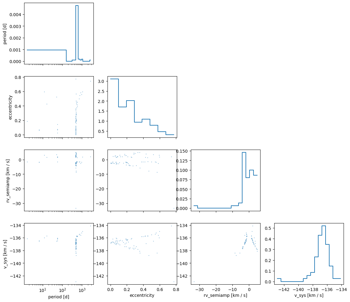
Right away we can notice a few things:

• First, the period distribution is highly multi-modal, with many well-separated modes corresponding to different orbital periods that are consistent with the data. This is a common feature of RV posteriors when the data are sparse or low signal-to-noise, and this is exactly why the rejection sampling method is so powerful for RV data: it can efficiently map out these complex posteriors in a way that MCMC methods would struggle with.

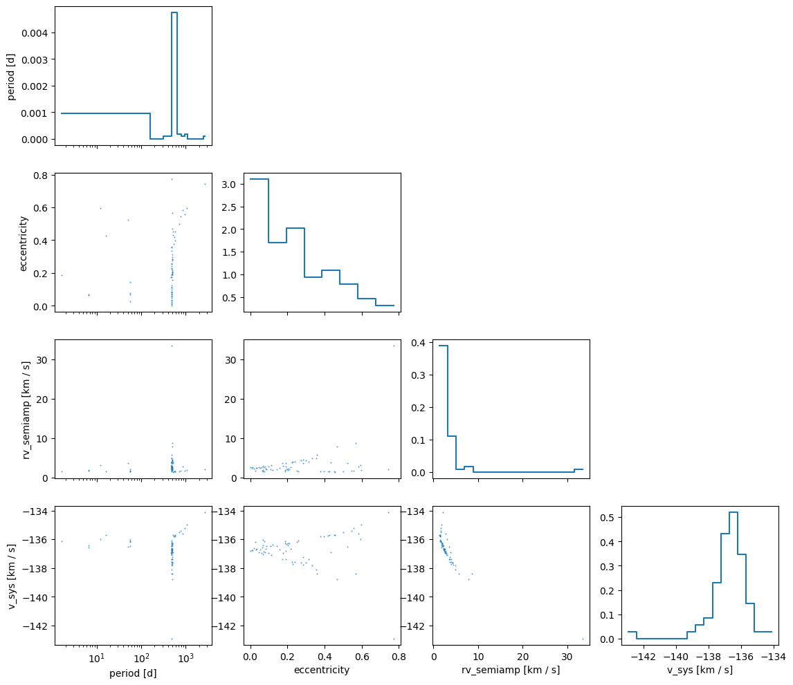
• Second, the RV semi-amplitude rv_semiamp has positive and negative values. This is a byproduct of the Gaussian prior we adopt on the semiamplitude in order to do the analytic marginalization. The negative values of rv_semiamp are equivalent to positive values with a 180 degree shift in the argument of periastron arg_peri. We can use the Samples.wrap_angles() method to wrap the angles to a more standard range (e.g. 0 to 360 degrees) and to keep physical parameters positive (e.g., semi-amplitude or, for astrometry, semimajor axis) if desired:

wrapped_samples = samples.wrap_angles()
axes = wrapped_samples.plot_corner(
    ["period", "eccentricity", "rv_semiamp", "v_sys"],
    visuals={"scatter": {"alpha": 0.75, "s": 2}},
)
for ax in axes.viz["plot"].isel(col_index=0).values.flat:
    if ax is not None:
        ax.set_xscale("log")

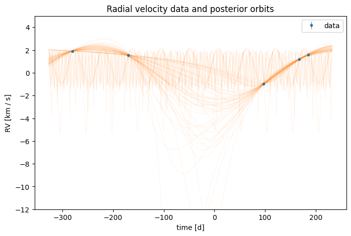
Another visualization that is often useful is to plot RV curves corresponding to the posterior samples over the data. We can do this using harv.plot.plot_rv():

fig, ax = plt.subplots(figsize=(8, 5))
ax = harv.plot.plot_rv(
    samples,
    data=data,
    n_samples=512,
    relative_to_t_ref=True,
    relative_to_median_v_sys=True,
    ax=ax,
)
ax.set(ylim=(-12, 5))

[(-12.0, 5.0)]

Next steps

With only a few observations, the posterior is highly multi-modal in orbital period.

In other settings, we may want to infer orbital parameters for data with more observations, higher signal-to-noise, or with a more constrained period. In these cases, the posterior may be less multi-modal and more amenable to MCMC sampling. Or, we may want to extend our model to add a more sophisticated noise model. Or, we may have data from multiple instruments or surveys that have instrumental / calibration offsets. We explore these cases in the next few tutorials.