Continuing the rejection-sampler posterior with MCMC¶

The rejection sampler in harv is designed to handle and map out the structure of complex, multi-modal RV posteriors. It can effectively survey the full prior volume and return a set of posterior samples even when the period is wildly multi-modal without having to consider convergence diagnostics or other metrics for assessing the quality of returned MCMC samples. But once we have isolated the mode(s) of interest (i.e., if the samples are unimodal in period), we usually want a dense posterior sampling with many independent samples for downstream uncertainty propagation. That’s where MCMC can help.

harv provides an interface to run standard MCMC using numpyro via the NumpyroSampler. This class builds a numpyro model from the same prior, parameterization, and extensions you used for rejection sampling, and can initialize from a Samples object outputted by a previous RejectionSampler run.

In this tutorial we’ll run rejection sampling on an APOGEE source with 28 visits and a clear orbit, including a Jitter extension to absorb any underestimated per-visit error bars, and use the returned sample(s) to start 4 MCMC chains of NUTS sampling to generate a denser sampling of the posterior.

We assume familiarity with the basic rejection-sampling workflow from the getting started tutorial.

Note

Later, we will run 4 MCMC chains. If you are running this locally, you can often run these in parallel. This requires telling JAX up front how many host devices to expose, which we do via numpyro.set_host_device_count(...) before importing JAX. Uncomment this code to run locally.

# import numpyro

# numpyro.set_host_device_count(4)

import arviz as az
import astropy.table as at
import jax
import matplotlib.pyplot as plt
import numpyro.distributions as dist
import quaxed.numpy as jnp
from unxt import Q

import harv
import harv.models as hm

jax.config.update("jax_enable_x64", True)

%matplotlib inline

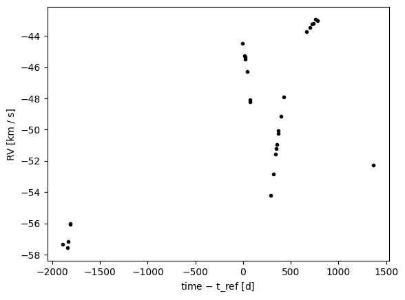
Loading the data¶

We use APOGEE DR17 visit RVs for source 2M03385429+4623449, which has 28 epochs and a clear, well-sampled orbital signal. This is exactly the regime where MCMC is worth the cost over rejection sampling alone.

tbl = at.Table.read("../data/apogeedr17-2M03385429+4623449.csv")

fdtype = jnp.float64
data = harv.RVData(
    time=Q(tbl["JD"].astype(fdtype), "day"),
    rv=Q(tbl["VHELIO"].astype(fdtype), "km/s"),
    rv_err=Q(tbl["VRELERR"].astype(fdtype), "km/s"),
)
data

RVData(
  time=Quantity(f64[28], unit='d'),
  t_ref=Quantity(weak_f64[], unit='d'),
  rv=Quantity(f64[28], unit='km / s'),
  rv_err=Quantity(f64[28], unit='km / s')
)

_ = data.plot(relative_to_t_ref=True)

../../_images/9190b6cb5c9ff152a93db740f91f9a0eb0d4d80cb25642e3328fe2515d5bce5b.png

Rejection sampling with a jitter extension¶

We set up the standard log-uniform period prior and etc. via default_prior(), and add a Jitter extension to allow extra (white) variance on top of the formal APOGEE error bars. The jitter parameter is sampled from a HalfNormal(0.5 km/s) prior. This is wide enough to allow up to ~few km/s of excess scatter if the data demand it, but with most prior mass at small jitter so we don’t over-inflate the errors when they’re already correct.

prior = hm.StandardRV().default_prior(
    period_min=Q(100.0, "day"),
    period_max=Q(2000.0, "day"),
    sigma_K0=Q(30.0, "km/s"),
    sigma_v0=Q(50.0, "km/s"),
    jitter=harv.QD(dist.HalfNormal(0.5), "km/s"),
)

model = harv.RVModel(extensions=(harv.Jitter(param_unit="km/s"),))

rej_sampler = harv.RejectionSampler(prior, model)
rej_samples = rej_sampler.run(
    data,
    n_prior_samples=10_000_000,
    max_posterior_samples=1024,
    seed=42,
)
len(rej_samples)

With 28 well-sampled epochs the period posterior should already be unimodal. And in fact, the rejection sampler returns only one sample because we used a very wide period prior. For your own use cases, the number of returned samples from the rejection sampler can depend strongly on the period prior. For example, if you use a restricted prior, you could end up with more samples for well-constrained cases like this one, but at the expense of missing other modes / orbital solutions in more complex cases (e.g., with fewer data points).

Let’s visualize the returned sample(s) from the rejection sampler:

fig, ax = plt.subplots(figsize=(8, 5))
ax = harv.plot.plot_rv(
    rej_samples,
    data=data,
    model=model,
    n_samples=128,
    relative_to_t_ref=True,
    relative_to_median_v_sys=True,
    ax=ax,
)

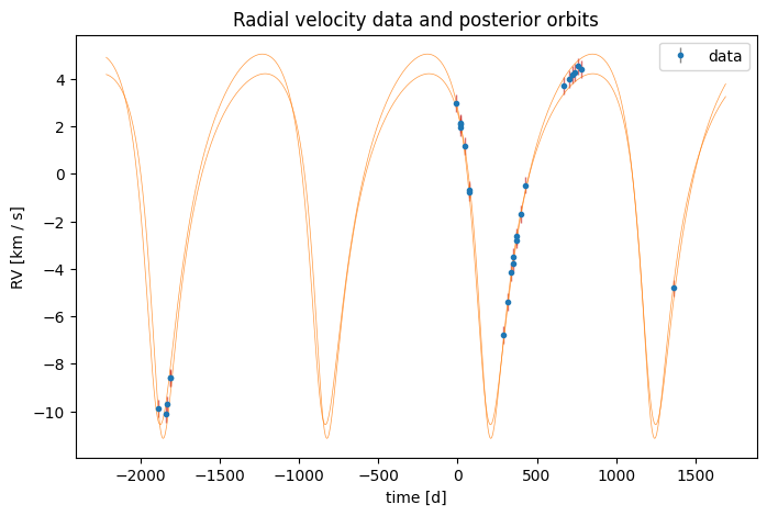
../../_images/67154b2f834e2903a5d2a496507e3e8594a7761bb83932912fb8f247c4d01361.png

Note that when jitter is included as an extension, the plotted data points are inflated (and drawn as red error bars by default) to include the median jitter value in addition to the formal error bars. In any case, for this data set, the returned sample from the rejection sampler looks like a good fit to the data.

Continuing with MCMC¶

Now we want a dense posterior sampling, so we will use the sample(s) from the rejection sampler to initialize the MCMC chains. NumpyroSampler takes the same prior and extensions we just used, and its run() method accepts an init_samples argument: rejection samples used to initialize each MCMC chain. With num_chains=4, the sampler picks 4 distinct rejection samples (cycling if there are fewer than 4) and uses them as the starting positions for 4 independent chains.

By default the sampler uses NUTS (no-U-turn HMC) with marginalized=True, meaning the linear parameters (rv_semiamp, v_sys) are analytically marginalized inside the likelihood and then conditionally sampled at the end so the returned Samples object still contains them. Only the nonlinear parameters (and any nonlinear extensions like jitter) are explored by HMC.

mcmc_sampler = harv.NumpyroSampler(prior, model)

mcmc_samples = mcmc_sampler.run(
    data,
    init_samples=rej_samples,
    num_chains=4,
    num_warmup=1000,
    num_samples=2000,
    seed=42,
)
mcmc_samples

/home/runner/work/harv/harv/src/harv/samplers/numpyro.py:427: UserWarning: There are not enough devices to run parallel chains: expected 4 but got 1. Chains will be drawn sequentially. If you are running MCMC in CPU, consider using `numpyro.set_host_device_count(4)` at the beginning of your program. You can double-check how many devices are available in your system using `jax.local_device_count()`.
  mcmc = _numpyro_infer.MCMC(

Samples(n_samples=8000, data_type='RVModel', parameters=10)

The returned Samples flattens the chain dimension by default — with num_chains=4 and num_samples=2000 we get \(4 \times 2000 = 8000\) samples. The chain count is preserved in the metadata in case we want to do per-chain diagnostics:

print("n_samples =", mcmc_samples.n_samples)
print("num_chains =", mcmc_samples.metadata["num_chains"])

n_samples = 8000
num_chains = 4

Numpyro internally returns an arviz-friendly xarray DataTree object. To get back the raw DataTree object, we can use the to_arviz() method on the returned Samples object:

We could use this object to assess the convergence of the MCMC sampling:

az.summary(dt)

	mean	sd	eti89_lb	eti89_ub	ess_bulk	ess_tail	r_hat	mcse_mean	mcse_sd
period	1036.38	0.65	1000	1000	6806	5415	1.00	0.008	0.0062
eccentricity	0.43178	0.00283	0.43	0.44	7537	5897	1.00	3.3e-05	2.6e-05
phase_peri	0.17718	0.00209	0.17	0.18	6002	4366	1.00	2.7e-05	2.1e-05
arg_peri	2.7345	0.0151	2.7	2.8	5843	4517	1.00	0.0002	0.00015
jitter	0.0756	0.0174	0.051	0.11	5628	4892	1.00	0.00023	0.0002
rv_semiamp	7.6453	0.034	7.6	7.7	8067	7589	1.00	0.00038	0.0003
v_sys	-47.3884	0.0218	-47	-47	7432	6845	1.00	0.00025	0.0002
log_period	3.01552	0.000274	3	3	6806	5415	1.00	3.3e-06	2.6e-06
t_peri	2.4579e+06	2.26	2.5e+06	2.5e+06	6015	4261	1.00	0.029	0.022
binary_mass_function	0.03522	0.000452	0.034	0.036	7986	7577	1.00	5.1e-06	4e-06

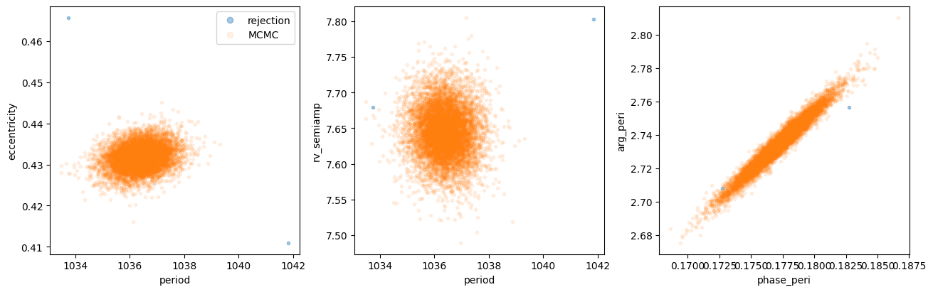
Step 3 — Comparing rejection and MCMC posteriors¶

Let’s overlay the rejection and MCMC posteriors. The MCMC chains should fill in a smooth, well-sampled posterior in the neighborhood of the rejection mode:

fig, axes = plt.subplots(1, 3, figsize=(13, 4), layout="constrained")

for ax, (xkey, ykey) in zip(
    axes,
    [("period", "eccentricity"), ("period", "rv_semiamp"), ("phase_peri", "arg_peri")],
    strict=True,
):
    rej_w = rej_samples.wrap_angles()
    mc_w = mcmc_samples.wrap_angles()
    ax.plot(rej_w[xkey].value, rej_w[ykey].value, ".", alpha=0.4, label="rejection")
    ax.plot(mc_w[xkey].value, mc_w[ykey].value, ".", alpha=0.1, label="MCMC")
    ax.set(xlabel=xkey, ylabel=ykey)
axes[0].legend(markerscale=2)

<matplotlib.legend.Legend at 0x7f1340f42900>

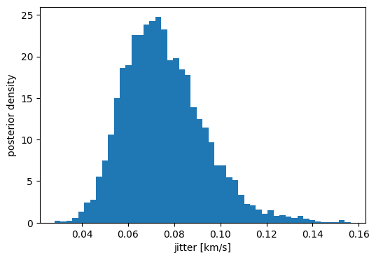
../../_images/776e9d9eca7ad698da62419111eec59e0a9460953bce2dd8d23a21f4d1937ffd.png

The jitter parameter is sampled by HMC alongside the orbital nonlinear parameters. Its marginal posterior tells us whether the formal APOGEE errors are sufficient or whether the data demand additional white-noise variance:

fig, ax = plt.subplots(figsize=(6, 4))
ax.hist(mcmc_samples["jitter"].to_value("km/s"), bins=50, density=True)
ax.set(xlabel="jitter [km/s]", ylabel="posterior density")

[Text(0.5, 0, 'jitter [km/s]'), Text(0, 0.5, 'posterior density')]

../../_images/8d6b844aebd9870ad246d056a1c048d9a6a2abca35585a7511c5100cb12d2394.png

Samples.summary returns median + 16th/84th percentile statistics for any subset of parameters — handy for reporting:

summ = mcmc_samples.wrap_angles().summary(
    ["period", "eccentricity", "arg_peri", "rv_semiamp", "v_sys", "jitter"]
)
print("Median values:")
for k, v in summ.items():
    print(f"{k}: {v['median']}")

Median values:
period: Quantity['time'](1036.38326446, unit='d')
eccentricity: Quantity['dimensionless'](0.4317612, unit='')
arg_peri: Quantity['angle'](2.73446889, unit='rad')
rv_semiamp: Quantity['speed'](7.64511663, unit='km / s')
v_sys: Quantity['speed'](-47.38789081, unit='km / s')
jitter: Quantity['speed'](0.07363848, unit='km / s')

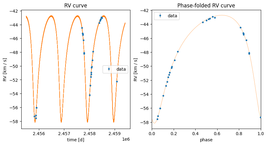
Finally, we will plot posterior orbit curves over the data using the MCMC samples:

fig, axes = plt.subplots(1, 2, figsize=(10, 5))
_ = harv.plot.plot_rv(
    mcmc_samples,
    data=data,
    extensions=model.extensions,
    n_samples=512,
    ax=axes[0],
)
_ = harv.plot.plot_rv(
    mcmc_samples,
    data=data,
    extensions=model.extensions,
    phase_fold_median=True,
    ax=axes[1],
)
axes[0].set(title="RV curve")
axes[1].set(title="Phase-folded RV curve")

[Text(0.5, 1.0, 'Phase-folded RV curve')]

../../_images/7528c35bc8e02ec44793e68e54ddf108ee02afad6bac0029530c12762468b16d.png