Extending the Keplerian model

In this tutorial, we show how to extend the base Keplerian model in harv to account for potential zero-point offsets between RV surveys or instruments, to complexify the noise model by adding a jitter (or, as we cover in a later tutorial, a Gaussian process background model), or to simultaneously model long-term trends in the data.

Each of these is supported via a harv.AbstractExtension that plugs into the same RejectionSampler workflow we used in the getting started tutorial. We recommend reading that tutorial first if you are new to harv.

This tutorial assumes familiarity with the basic RVData / HarvPrior / RejectionSampler workflow introduced in the previous tutorials.

import astropy.table as at
import jax
import matplotlib.pyplot as plt
import numpyro.distributions as dist
from unxt import Q

import harv
import harv.models as hm

jax.config.update("jax_enable_x64", True)

%matplotlib inline

1. Multi-survey data with instrumental offsets

When two spectrographs observe the same star, the reported radial velocities may differ by an offset because of differences in the wavelength solution or other instrumental effects. If we naively concatenate the two datasets and fit a single Keplerian model, this offset will bias the inferred parameters (especially the systemic velocity and eccentricity) and could lead to poor performance of the sampler.

harv supports simultaneously inferring instrumental offsets through the MultiSurveyOffset extension, which adds one linear parameter per instrument (beyond the adopted reference instrument). That is, you specify which survey or dataset should be treated as the reference, and infer a per-instrument additive offset that is analytically marginalized along with v_sys and rv_semiamp.

For this example we’ll use simulated data so we know the true parameters. We’ll imagine that we have two surveys, “survey1” and “survey2”, that observed the same star. We can load the data for each survey and store them together in a single SourceData object:

tbl = at.Table.read("../data/simulated-multi-survey-data.fits")
survey1_data = harv.RVData(
    time=Q(tbl["time"][tbl["survey"] == "survey1"].astype("f8"), "day"),
    rv=Q(tbl["rv"][tbl["survey"] == "survey1"].astype("f8"), "km/s"),
    rv_err=Q(tbl["rv_err"][tbl["survey"] == "survey1"].astype("f8"), "km/s"),
)

survey2_data = harv.RVData(
    time=Q(tbl["time"][tbl["survey"] == "survey2"].astype("f8"), "day"),
    rv=Q(tbl["rv"][tbl["survey"] == "survey2"].astype("f8"), "km/s"),
    rv_err=Q(tbl["rv_err"][tbl["survey"] == "survey2"].astype("f8"), "km/s"),
)

source_data = harv.SourceData(survey1=survey1_data, survey2=survey2_data)
source_data

SourceData(
  _datasets={
    'survey1':
    RVData(
      time=Quantity(f64[16], unit='d'),
      t_ref=Quantity(f64[], unit='d'),
      rv=Quantity(f64[16], unit='km / s'),
      rv_err=Quantity(f64[16], unit='km / s')
    ),
    'survey2':
    RVData(
      time=Quantity(f64[12], unit='d'),
      t_ref=Quantity(f64[], unit='d'),
      rv=Quantity(f64[12], unit='km / s'),
      rv_err=Quantity(f64[12], unit='km / s')
    )
  }
)

SourceData.plot draws each component on a single axes with distinct colors and a legend, so we can see at a glance whether the two datasets agree on the systemic velocity and the orbital signal.

_ = source_data.plot()

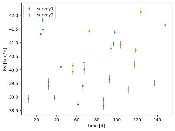
Here, the offset must be small, because it is not clearly visible by eye between the two simulated datasets. Let’s see if we can infer it with harv.

Building the prior and the model

The MultiSurveyOffset extension needs a precomputed indicator matrix that says which observation came from which instrument. The SourceData.indicator_data_by_type helper constructs this for us: given a reference instrument, it returns

• stacked_data — a single RVData with all observations concatenated,

• indicator — a (n_obs, n_non_reference) 0/1 matrix with one column per non-reference instrument, and

• instrument_names — the column ordering for indicator.

We pick survey1 as the reference (its offset is absorbed by v_sys) and put a Gaussian prior on the offset of survey2 with respect to the reference. The simplest way to declare the offset prior is to pass it as a keyword argument to default_prior() whose name matches the non-reference instrument:

stacked_data, indicator, instrument_names = source_data.indicator_data_by_type(
    harv.RVData, reference="survey1"
)
stacked_data

RVData(
  time=Quantity(f64[28], unit='d'),
  t_ref=Quantity(weak_f64[], unit='d'),
  rv=Quantity(f64[28], unit='km / s'),
  rv_err=Quantity(f64[28], unit='km / s')
)

indicator

Array([[0.],
       [0.],
       [0.],
       [0.],
       [0.],
       [0.],
       [0.],
       [0.],
       [0.],
       [0.],
       [0.],
       [0.],
       [0.],
       [0.],
       [0.],
       [0.],
       [1.],
       [1.],
       [1.],
       [1.],
       [1.],
       [1.],
       [1.],
       [1.],
       [1.],
       [1.],
       [1.],
       [1.]], dtype=float64)

instrument_names

('survey2',)

prior = hm.StandardRV().default_prior(
    period_min=Q(1.0, "day"),
    period_max=Q(3000.0, "day"),
    sigma_K0=Q(30.0, "km/s"),
    sigma_v0=Q(50.0, "km/s"),
    # One offset prior per non-reference instrument. The keyword name must
    # match the instrument name passed to SourceData(...).
    survey2=harv.QD(dist.Normal(0.0, 1.0), "km/s"),
)

Because the offset is a linear extension parameter, RejectionSampler merges it into the effective linear prior automatically and analytically marginalizes it along with rv_semiamp and v_sys. We build an RVModel with the extension and pass both to the sampler:

model = harv.RVModel(
    extensions=(harv.MultiSurveyOffset(indicator, instrument_names, "km/s"),),
)

sampler = harv.RejectionSampler(prior, model)
samples = sampler.run(
    stacked_data, n_prior_samples=10_000_000, max_posterior_samples=1024, seed=42
)
samples

Samples(n_samples=7, data_type='RVModel', parameters=10)

The returned Samples object now has an extra entry for each non-reference instrument’s offset (survey2 in this case), in addition to the standard orbital parameters:

samples.keys()

['arg_peri',
 'eccentricity',
 'period',
 'phase_peri',
 'rv_semiamp',
 'survey2',
 'v_sys',
 'log_period',
 't_peri',
 'binary_mass_function']

Let’s visualize the posterior samples:

axes = samples.wrap_angles().plot_corner(
    ["period", "eccentricity", "rv_semiamp", "v_sys", "survey2"],
)

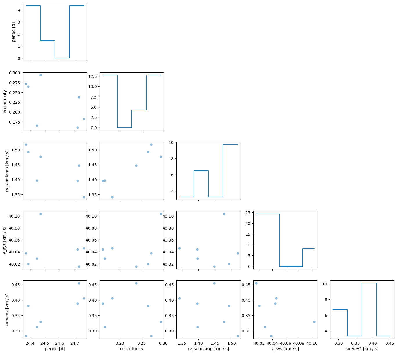
Only a few samples were returned, but the offset (survey2) is clearly detected and has a value of around 0.4 km/s (based on these samples).

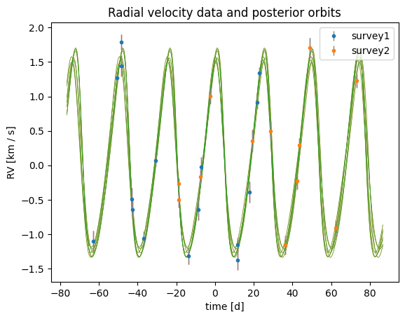
harv.plot.plot_rv() recognizes the MultiSurveyOffset extension when the sampler’s extensions are passed in: it will plot each instrument in its own color and shift the non-reference data points by the median posterior offset (apply_median_offsets=True, the default).

ax = harv.plot.plot_rv(
    samples,
    data=source_data,
    model=model,
    n_samples=128,
    relative_to_t_ref=True,
    relative_to_median_v_sys=True,
    apply_median_offsets=True,
)

From here, we could use these returned posterior samples to run an MCMC sampler to better characterize the posterior distribution. We show how to do this in the next tutorial, Continuing the rejection-sampler posterior with MCMC.

2. Jitter: handling underestimated uncertainties

Reported per-observation RV uncertainties are often optimistic (i.e., underestimated). Pipelines often do not propagate every systematic, and astrophysical noise (granulation, oscillations, etc.) is not captured by the formal photon-noise errors. If we trust the formal errors, the model is forced to fit every fluctuation as a real Keplerian signal, and we can get spurious tight constraints on the orbital parameters but bad likelihood (or reduced \(\chi^2\)) values.

A standard remedy to handle these issues is to add a constant jitter term \(s\) in quadrature to the per-observation variance:

\[\sigma_\mathrm{eff}^2 = \sigma_\mathrm{obs}^2 + s^2\]

where \(s\) is sampled jointly with the other parameters. In harv this is supported via the Jitter extension. We declare a prior on jitter (typically a HalfNormal since it is a positive scale) and pass the extension to the sampler. But note that this is a nonlinear extension, so this does increase the dimensionality of the parameter space. However, in contrast to other parameters, adding a jitter often will improve the performance of the sampler by allowing it to find more samples with good likelihood values.

We’ll demonstrate this on a high signal-to-noise (SNR ~ 1000) target from APOGEE. Bright targets in APOGEE often have underestimated visit RV uncertainties.

tbl = at.Table.read("../data/apogeedr17-2M00073823+7353217.csv")

data = harv.RVData(
    time=Q(tbl["JD"].astype("f8"), "day"),
    rv=Q(tbl["VHELIO"].astype("f8"), "km/s"),
    rv_err=Q(tbl["VRELERR"].astype("f8"), "km/s"),
)
_ = data.plot(relative_to_t_ref=True)

To enable jitter we pass two pieces:

1. a prior named jitter to default_rv: In this case, we use a HalfNormal distribution with an arbitrary scale (you could set this in a more principled way based on your own assumptions of the noise floor, or you could even infer this as a function of SNR from the population of stars observed by APOGEE!), and

2. a Jitter(param_unit="km/s") extension to the sampler.

prior_jitter = hm.StandardRV().default_prior(
    period_min=Q(0.5, "day"),
    period_max=Q(3000.0, "day"),
    sigma_K0=Q(30.0, "km/s"),
    sigma_v0=Q(50.0, "km/s"),
    jitter=harv.QD(dist.HalfNormal(1.0), "km/s"),
)
rv_model_jitter = harv.RVModel(extensions=(harv.Jitter(param_unit="km/s"),))

sampler_jitter = harv.RejectionSampler(prior_jitter, rv_model_jitter)
samples_jitter = sampler_jitter.run(
    data, n_prior_samples=10_000_000, max_posterior_samples=1024, seed=42
)
len(samples_jitter)

20

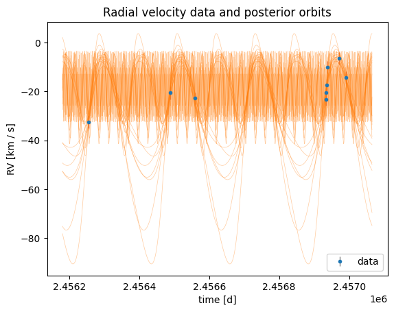
Here only a handful of samples are returned: let’s visualize them as orbits over the data

harv.plot.plot_rv(samples_jitter, data=data, model=rv_model_jitter, n_samples=128)

<Axes: title={'center': 'Radial velocity data and posterior orbits'}, xlabel='time [d]', ylabel='RV [km / s]'>

Let’s compare to a model that does not include jitter, to see how the inferred orbital parameters change

prior_no_jitter = hm.StandardRV().default_prior(
    period_min=Q(0.5, "day"),
    period_max=Q(3000.0, "day"),
    sigma_K0=Q(30.0, "km/s"),
    sigma_v0=Q(50.0, "km/s"),
)
samples_no_jitter = harv.RejectionSampler(prior_no_jitter, harv.RVModel()).run(
    data, n_prior_samples=10_000_000, max_posterior_samples=1024, seed=42
)
len(samples_no_jitter)

1

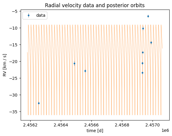
Without jitter, only 1 sample is returned, and it looks very eccentric and does not fit the data well. This is a generic issue when the uncertainties are underestimated: the sampler is forced to find a single solution that fits every possible fluctuation in the data, which often leads to spurious eccentricity and poor likelihood values.

harv.plot.plot_rv(samples_no_jitter, data=data, n_samples=128)

<Axes: title={'center': 'Radial velocity data and posterior orbits'}, xlabel='time [d]', ylabel='RV [km / s]'>

3. Long-term polynomial trend

A common configuration for triple-star systems is a short-period inner binary with an outer, long-period / tertiary. Over a time baseline that is shorter than the outer orbit’s period, the outer companion produces a roughly linear or polynomial trend in the systemic velocity that the inner Keplerian model can’t absorb. If we fit only a single Keplerian, the linear trend leaks into biased eccentric or otherwise strange inner orbital parameter solutions.

The MonomialTrend extension adds polynomial terms (t - t_ref)^k for k = 1..order as additional linear parameters of the design matrix (so they’re analytically marginalized just like v_sys). The names of the trend parameters are trend_1, trend_2, … We also plan to add support for other polynomial bases (e.g., Legendre polynomials) in the future.

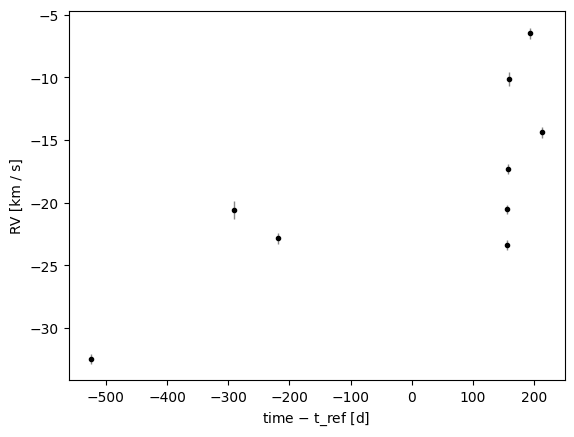
For this example, we simulated the radial velocity signal of a triple system in which we have the radial velocities of the most massive star (the primary). The inner binary has a period of about 25 day and the outer companion has a period of about 1000 days. Over the time baseline of the simulated data (~300 days), the outer companion induces a roughly quadratic trend in the systemic velocity, but this trend is not immediately apparent in the data by eye.

tbl = at.Table.read("../data/simulated-long-trend.fits")
trend_data = harv.RVData(
    time=Q(tbl["time"].astype("f8"), "day"),
    rv=Q(tbl["rv"].astype("f8"), "km/s"),
    rv_err=Q(tbl["rv_err"].astype("f8"), "km/s"),
)
_ = trend_data.plot(relative_to_t_ref=True)

We’ll start by modeling the data with a single Keplerian and no trend, to see how the inferred parameters are biased by the unmodeled trend:

prior_no_trend = hm.StandardRV().default_prior(
    period_min=Q(0.5, "day"),
    period_max=Q(1e3, "day"),
    sigma_K0=Q(30.0, "km/s"),
    sigma_v0=Q(50.0, "km/s"),
)
samples_no_trend = harv.RejectionSampler(prior_no_trend, harv.RVModel()).run(
    trend_data, n_prior_samples=10_000_000, max_posterior_samples=512, seed=42
)

fig, axes = plt.subplots(1, 2, figsize=(12, 5), sharey=True)
_ = harv.plot.plot_rv(samples_no_trend, data=trend_data, n_samples=128, ax=axes[0])
_ = harv.plot.plot_rv(
    samples_no_trend, data=trend_data, phase_fold_median=True, ax=axes[1]
)
[ax.set_title("") for ax in axes]

[Text(0.5, 1.0, ''), Text(0.5, 1.0, '')]

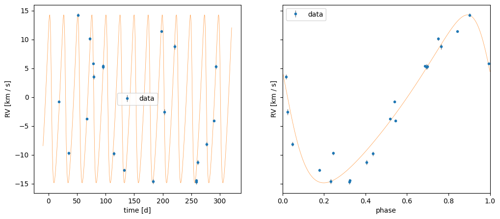
Here we can see from the phase-folded plot that the inferred orbit does not look like a very good fit to the data, even though the time-series plot looks reasonable. Let’s now include a quadratic trend in the model and see how the inferred parameters change.

The MonomialTrend extension takes the polynomial order (1 for a linear drift, 2 for quadratic, etc.) and a time_unit for unit-stripping. Because the trend parameters are linear, we declare priors on them via the same default_rv(...) kwarg mechanism:

trend = harv.MonomialTrend(order=2, time_unit="day", obs_unit="km/s")

prior_trend = hm.StandardRV().default_prior(
    period_min=Q(0.5, "day"),
    period_max=Q(1e3, "day"),  # short-period inner orbit
    sigma_K0=Q(30.0, "km/s"),
    sigma_v0=Q(50.0, "km/s"),
    trend_1=harv.QD(dist.Normal(0.0, 0.5), "km/s"),  # km/s per day
    trend_2=harv.QD(dist.Normal(0.0, 0.05), "km/s"),  # km/s per day^2
)

Now we can run the sampler with the trend extension:

trend_model = harv.RVModel(extensions=(trend,))
sampler_trend = harv.RejectionSampler(prior_trend, trend_model)
samples_trend = sampler_trend.run(
    trend_data, n_prior_samples=10_000_000, max_posterior_samples=512, seed=42
)
len(samples_trend)

1

fig, axes = plt.subplots(1, 2, figsize=(12, 5), sharey=True)
_ = harv.plot.plot_rv(
    samples_trend, data=trend_data, n_samples=128, ax=axes[0], model=trend_model
)
_ = harv.plot.plot_rv(
    samples_trend,
    data=trend_data,
    phase_fold_median=True,
    ax=axes[1],
    model=trend_model,
)
[ax.set_title("") for ax in axes]

[Text(0.5, 1.0, ''), Text(0.5, 1.0, '')]

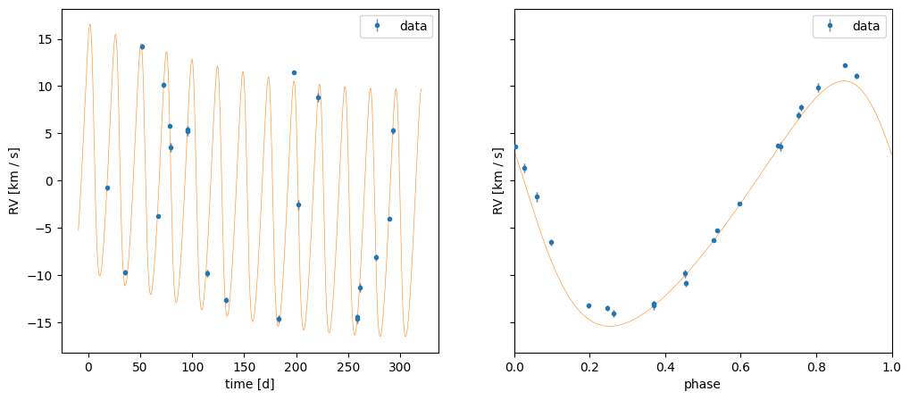
We can see that the returned samples here have a similar period, but a different amplitude and eccentricity. The trend also picks up a clear long-period signal, which de-biases the inner orbit’s parameters and allows it to fit the data much better.

Combining extensions

All model extensions compose: pass a tuple of extensions to the sampler in the order you want them applied. For example, a multi-survey fit with both a per-instrument offset, a global jitter, and a long-term linear trend is just

extensions = (
    harv.MultiSurveyOffset(indicator, instrument_names, "km/s"),
    harv.Jitter(param_unit="km/s"),
    harv.MonomialTrend(order=1, time_unit="day", obs_unit="km/s"),
)

with matching jitter=..., trend_1=..., and <instrument>=... priors passed as kwargs to default_rv. The AbstractExtension interface is intentionally minimal — only extra_params, modify_design_matrix, and modify_covariance — so writing a new extension (e.g. a custom kernel, an alternative trend basis, or a calibration term tied to an external regressor) is straightforward and slots into the same sampler workflow shown here.